13. Volume
b1. Solids of Revolution
If a region in the \(xy\)-plane is rotated about some axis, it sweeps out a solid called a Solid of Revolution. For example, here are four regions in the \(xy\)-plane and the solids swept out when they are rotated about the \(x\)-axis or the \(y\)-axis:
-
Area below \(y=f(x)\) above \(x\)-axis rotated about \(x\)-axis
and \(y\)-axis:
Region 1 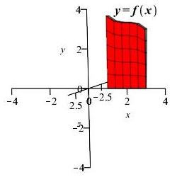
Region 1 \(x\)-axis Region 1 \(y\)-axis -
Area below \(y=f(x)\) above \(y=g(x)\) rotated
about \(x\)-axis and \(y\)-axis:
Region 2 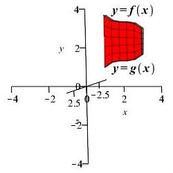
Region 2 \(x\)-axis Region 2 \(y\)-axis -
Area left of \(x=f(y)\) right of \(y\)-axis rotated about
\(x\)-axis and \(y\)-axis:
Region 3 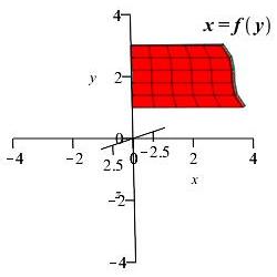
Region 3 \(x\)-axis Region 3 \(y\)-axis -
Area left of \(x=f(y)\) right of \(x=g(y)\)
rotated about \(x\)-axis and \(y\)-axis:
Region 4 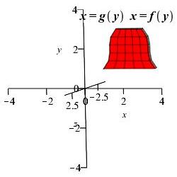
Region 4 \(x\)-axis Region 4 \(y\)-axis
As with all integration problems, we chop the solid up into small pieces, approximate the volume of each piece, add them up and take the limit as the number of pieces gets large and the size of each piece gets small.
For regions 1 and 2, the region is defined in terms of functions of \(x\). So we chop up the \(x\)-interval into small pieces of length \(\Delta x\).
For regions 3 and 4, the region is defined in terms of functions of \(y\). So we chop up the \(y\)-interval into small pieces of length \(\Delta y\).
Here are the corresponding small pieces of the regions and the corresponding small pieces of the volumes of revolution:
-
Area below \(y=f(x)\) above \(x\)-axis rotated about \(x\)-axis
and \(y\)-axis:
Rectangle 1 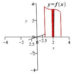
Rectangle 1 \(x\)-axis
Rectangle 1 \(y\)-axis
-
Area below \(y=f(x)\) above \(y=g(x)\) rotated
about \(x\)-axis and \(y\)-axis:
Rectangle 2 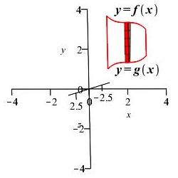
Rectangle 2 \(x\)-axis
Rectangle 2 \(y\)-axis
-
Area left of \(x=f(y)\) right of \(y\)-axis rotated about
\(x\)-axis and \(y\)-axis:
Rectangle 3 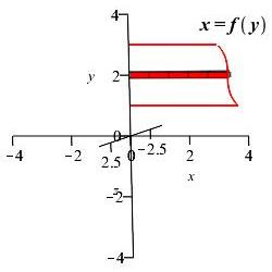
Rectangle 3 \(x\)-axis
Rectangle 3 \(y\)-axis
-
Area left of \(x=f(y)\) right of \(x=g(y)\)
rotated about \(x\)-axis and \(y\)-axis:
Rectangle 4 
Rectangle 4 \(x\)-axis
Rectangle 4 \(y\)-axis
Notice that:
Rectangles 1x and 3y rotate into
thin disks,
Rectangles 2x and 4y rotate into
thin washers and
Rectangles 1y, 2y, 3x and 4x rotate into
thin cylinders.
(Thin cylinders are also called cylindrical shells.)
The integrals are slightly different in each of the three cases.
Do not try to memorize which shape arises from each choice of integration variable and which way it is rotated.
Rather, on subsequent pages, we will explain how to distinguish between them. On the next page we will discuss the general procedure for how to determine the shape. Then on subsequent pages, we will discuss thin disks, thin washers and thin cylinders.
Heading
Placeholder text: Lorem ipsum Lorem ipsum Lorem ipsum Lorem ipsum Lorem ipsum Lorem ipsum Lorem ipsum Lorem ipsum Lorem ipsum Lorem ipsum Lorem ipsum Lorem ipsum Lorem ipsum Lorem ipsum Lorem ipsum Lorem ipsum Lorem ipsum Lorem ipsum Lorem ipsum Lorem ipsum Lorem ipsum Lorem ipsum Lorem ipsum Lorem ipsum Lorem ipsum