26. Stokes' Theorem
Let \(S\) be a nice surface in \(\mathbb{R}^3\) with a nice properly oriented boundary, \(\partial S\), and let \(\vec{F}\) be a nice vector field on \(S\). Then \[ \iint_S \vec{\nabla}\times\vec{F}\cdot d\vec{S} =\oint_{\partial S} \vec{F}\cdot d\vec{s} \] Each piece of the boundary of the surface must be traversed counterclockwise as seen from the tip of the normal vector to the surface.
d. Applications
3. Path Independence
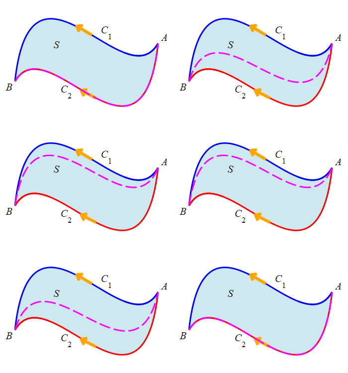
Suppose \(C_1\) and \(C_2\) are two open curves which start at \(A\) and end at \(B\). We say that \(C_1\) can be continuously deformed into \(C_2\) if there is a surface \(S\) whose boundary is \(\partial S=C_1-C_2\). This means that the boundary of \(S\) may be traversed with the proper counterclockwise orientation by traveling forward along \(C_1\) and then backward along \(C_2\).
In the figure, notice that \(C_2\) is traversed in the same direction as \(C_1\), but needs to be reversed to complete the boundary of \(S\) with the normal pointing out of the page.
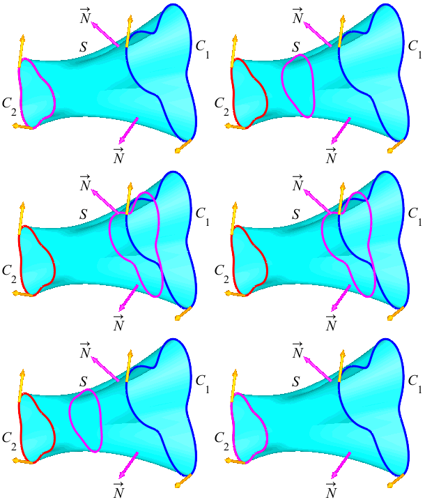
Similarly, suppose \(C_1\) and \(C_2\) are two closed curves. We say that \(C_1\) can be continuously deformed into \(C_2\) if there is a surface \(S\) whose boundary is \(\partial S=C_1-C_2\). This means that the boundary of \(S\) consists of two curves \(C_1\) and \(C_2\) with \(C_1\) traversed forwards and \(C_2\) traversed backwards.
In the figure, notice that \(C_2\) is traversed in the same direction as \(C_1\), but needs to be reversed to complete the boundary of \(S\) with the normal as shown.
In either case, \(\partial S=C_1-C_2\), and so Stokes' Theorem says \[ \iint_S \vec{\nabla}\times\vec{F}\cdot d\vec{S} =\oint_{\partial S} \vec{F}\cdot d\vec{s} =\oint_{C_1} \vec{F}\cdot d\vec{s} -\oint_{C_2} \vec{F}\cdot d\vec{s} \] This may be rewritten as \[ \int_{C_1} \vec{F}\cdot d\vec{s} =\int_{C_2} \vec{F}\cdot d\vec{s} +\iint_S \vec{\nabla}\times\vec{F}\cdot d\vec{S} \qquad\qquad \text{(*)} \] In other words, to compute \(\displaystyle \int_{C_1} \vec{F}\cdot d\vec{s}\), you may alternatively compute \(\displaystyle \int_{C_2} \vec{F}\cdot d\vec{s}\) and \(\displaystyle \iint_S \vec{\nabla}\times\vec{F}\cdot d\vec{S}\), if that is easier.
Suppose that \(\vec F\) is a vector field satisfying \[ \int_{C_1} \vec{F}\cdot d\vec{s} =\int_{C_2} \vec{F}\cdot d\vec{s} \] whenever \(C_1\) can be continuously deformed into \(C_2\). Then we say \(\vec F\) has path independent line integrals.
In the special case that \(\vec\nabla\times\vec{F}=\vec 0\), then equation (*) says \(\vec F\) has path independent line integrals.
Let's compute a line integral in two different ways: Once directly and once using Stokes' Theorem and the relation \((*)\).
Compute the integral
\(\displaystyle \int_{C_1} \vec{F}\cdot d\vec{s}\) for
\(\displaystyle \vec{F}=\langle 2x+y,y-2\rangle\)
over the semi-circle \(C_1\) given by \(x^2+y^2=16\) counterclockwise from
\(A=(4,0)\) to \(B=(-4,0)\).
Compute it in two different ways:
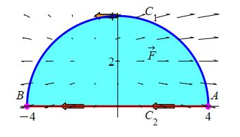
(1) directly along the curve \(C_1\), shown in blue, and
(2) using the relation \((*)\) where \(C_2\) is the straight line segment
from \(A\) to \(B\), shown in red,
and \(S\) is the region inside the semi-circle inside \(x^2+y^2=16\)
for \(y\ge0\), shown in cyan.
The semicircle \(C_1\) is parameterized as \(\vec{r}(\theta)=(4\cos\theta, 4\sin\theta)\) for \(0 \le \theta \le \pi\). So the velocity is \[ \vec{v}(\theta) =\langle-4\sin\theta, 4\cos\theta\rangle. \] This is properly parametrized counterclockwise. Next we evaluate the vector field on the curve: \[ \vec{F} =\langle 2x+y,y-2\rangle =\langle 8\cos\theta+4\sin\theta, 4\sin\theta- 2\rangle \] So the integral is: (Be careful with the range of \(\theta\).) \[\begin{aligned} \int_{C_1} \vec{F}\cdot d\vec{s} &=\int_0^\pi \vec{F}\cdot\vec{v}\,d\theta \\ &=\int_0^\pi (-32\sin\theta\cos\theta- 16\sin^2\theta +16\sin\theta\cos\theta- 8\cos\theta)\,d\theta \\ &=\int_0^\pi (-16\sin\theta\cos\theta - 16\dfrac{1-\cos(2\theta)}{2}-8\cos\theta)\,d\theta \\ &=\left[- 8\sin^2\theta - 8\left(\theta- \dfrac{\sin(2\theta)}{2}\right) - 8\sin\theta\right]_0^\pi =- 8\pi \end{aligned}\]
The line \(C_2\) may be parameterized as:
\(\vec{r}(t)=(t, 0)\)
for \(-4\le t \le4\).
The velocity is:
\(\vec{v}=(1, 0)\).
This points to the right, but we need it to point to the left. So we reverse it:
\[
\vec{v}=(- 1, 0)
\]
The vector field on the line is:
\[
\vec{F}(\vec{r}(t))
=\langle 2x+y,y-2\rangle
=\langle 2t,- 2\rangle.
\]
So the line integral is:
\[
\int_{C_2} \vec{F}\cdot d\vec{s}
=\int_{-4}^4 \vec{F}\cdot\vec{v}\,dt
=\int_{-4}^4 (-2t)\,dt
=\left[\rule{0pt}{10pt}-t^2\right]_{-4}^4=0
\]
To use the formulas for Stokes' Theorem, we need to work in
\(\mathbb{R}^3\). So the surface is the semi-circle \(x^2+y^2\le16\)
for \(y\ge0\) with \(z=0\). It is best to work in cylindrical coordinates.
So the surface may be parametrized as:
\(\vec{R}=(r\cos\theta, r\sin\theta, 0)\)
for which the normal is \(\vec{N}=(0,0,r)\). This points up along the
\(z\)-axis. So the curve must be traversed counterclockwise which
\(\partial S=C_1-C_2\) is.
The curl of the vector field \(\vec{F}=\langle 2x+y,y-2,0\rangle\) in rectangular coordinates is: \[ \vec{\nabla}\times\vec{F} =\begin{vmatrix} \hat{\imath} & \hat{\jmath} & \hat{k} \\ \partial_x & \partial_y & \partial_z \\ 2x+y & y-2 & 0 \\ \end{vmatrix} =\langle 0, 0,-1\rangle \] So the surface integral over \(S\) is: (Be careful with the range of \(\theta\).) \[\begin{aligned} \iint_S &\vec{F}\cdot d\vec{S} =\int_0^\pi\int_0^4 \vec{F}\cdot\vec{N}\,dr\,d\theta \\ &=\int_0^\pi\int_0^4 (-r)\,dr\,d\theta =-\pi\left[\dfrac{r^2}{2}\right]_0^4 =-8\pi \end{aligned}\] That was easy!
Finally we add the two integrals to get our answer: \[ \int_{C_1} \vec{F}\cdot d\vec{S} =\int_{C_2} \vec{F}\cdot d\vec{S} +\iint_S \vec{\nabla}\times\vec{F}\cdot d\vec{S} =0-8\pi=-8\pi \]
Notice the answers are the same. Clearly the integrals over the line and area were easier than the integral over the semi-circle.
Consider the integral \(\displaystyle I=\int_A^B \vec{F}\cdot d\vec{s}\) for \(\displaystyle \vec{F}=\langle e^x, e^y, e^z \rangle\), where \(A=(0,0,0)\) and \(B=(1,2,3)\).
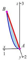
Compute the integral \(I\) along the parabola \(P\) parametrized by \(\vec{r}(t)=(t, 2t^2, 3t^2)\), for \(0\le t\le 1\), shown in blue.
Compute the integral \(I\) along the line \(L\) parametrized by \(\vec{r}(t)=(t, 2t, 3t)\), for \(0\le t\le 1\), shown in red.
\(\displaystyle I=\int_0^1 \vec{F}\cdot\vec{v}\,dt\)
\(\displaystyle I=e+e^2+e^3-3\)
The parabola \(P\), parametrized by \(\vec{r}(t)=(t, 2t^2, 3t^2)\), has velocity \(\vec{v}(t)=(1, 4t, 6t)\). On the parabola, the vector field is: \[ \vec{F}=\langle e^x, e^y, e^z \rangle =\langle e^{\small t}, e^{\small 2t^2}, e^{\small 3t^2} \rangle \] Their dot product is: \[ \vec{F}\cdot\vec{v}=e^{\small t}+4te^{\small 2t^2}+6te^{\small 3t^2} \] So the line integral is: \[\begin{aligned} I&=\int_A^B \vec{F}\cdot d\vec{s} =\int_0^1 \vec{F}\cdot\vec{v}\,dt \\ &=\int_0^1 \left(e^{\small t}+4te^{\small 2t^2}+6te^{\small 3t^2}\right)\,dt \\ &=\left[e^{\small t}+e^{\small 2t^2}+e^{\small 3t^2}\right]_0^1 =e+e^2+e^3-3 \end{aligned}\]
\(\displaystyle I=\int_0^1 \vec{F}\cdot\vec{v}\,dt\)
\(\displaystyle I=e+e^2+e^3-3\)
The line \(L\), parametrized by \(\vec{r}(t)=(t, 2t, 3t)\), has velocity \(\vec{v}(t)=(1,2,3)\). On the line, the vector field is: \[ \vec{F}=\langle e^x, e^y, e^z \rangle =\langle e^{\small t}, e^{\small 2t}, e^{\small 3t} \rangle \] Their dot product is: \[ \vec{F}\cdot\vec{v}=e^{\small t}+2e^{\small 2t}+3e^{\small 3t} \] So the line integral is: \[\begin{aligned} I&=\int_A^B \vec{F}\cdot d\vec{s} =\int_0^1 \vec{F}\cdot\vec{v}\,dt \\ &=\int_0^1 \left(e^{\small t}+2e^{\small 2t}+3e^{\small 3t}\right)\,dt \\ &=\left[e^{\small t}+e^{\small 2t}+e^{\small 3t}\right]_0^1 =e+e^2+e^3-3 \end{aligned}\] The answer is the same!
Why do the answers to (2a) and (2b) have be the same?
See the definition of path independence above. Compute \(\vec\nabla\times\vec F\).
Since, \(\vec\nabla\times\vec F=\vec 0\), the vector field has path independent line integrals. The integral \(I\) will have the same value on any curve from \(A\) to \(B\).
Since the integral \(I\) is the same for the parabola \(P\) and the line \(L\), we suspect that \(\vec F\) has path independent line integrals. To check, we compute its curl: \[\begin{aligned} \vec{\nabla}\times\vec{F} &=\begin{vmatrix} \hat\imath & \hat\jmath & \hat k \\ \partial_x & \partial_y & \partial_z \\ e^x & e^y & e^z \end{vmatrix} \\ &=\hat\imath(0)-\hat\jmath(0)+\hat k(0) =\vec 0 \end {aligned}\] Since, \(\vec\nabla\times\vec F=\vec 0\), the vector field \(\vec F\), has path independent line integrals. So the integral \(I\) will have the same value on any curve from \(A\) to \(B\).
In the chapter on the Fundamental Theorem of Calculus for Curves, we also discussed path independence. Find a scalar potential for \(\vec F\) and use the FTCC to compute \(I\) without specifying any curve. Which of the three methods was easiest (2a), (2b) or (2d)?
Solve \(\vec\nabla f=\vec F\). Then \[ \int_A^B \vec{F}\cdot d\vec{s} =\int_A^B \vec\nabla f\cdot d\vec{s} =f(B)-f(A) \]
The scalar potential is \(f=e^x+e^y+e^z\).
\(\displaystyle
I=e+e^2+e^3-3\)
To find a scalar potential for \(\vec{F}=\langle e^x, e^y, e^z \rangle\), we need to find a single function \(f\) satisfying \(\vec\nabla f=\vec F\), or: \[ \partial_x f=e^x \qquad \partial_y f=e^y \qquad \partial_z f=e^z \] A common solution is \(f=e^x+e^y+e^z\). By the FTCC, the integral is \[\begin{aligned} I&=\int_A^B \vec{F}\cdot d\vec{s} =\int_A^B \vec\nabla f\cdot d\vec{s} \\ &=f(B)-f(A)=f(1,2,3)-f(0,0,0) =e+e^2+e^3-3 \end{aligned}\]
The FTCC was clearly the easiest. But only because it was easy to find the scalar potential.
Heading
Placeholder text: Lorem ipsum Lorem ipsum Lorem ipsum Lorem ipsum Lorem ipsum Lorem ipsum Lorem ipsum Lorem ipsum Lorem ipsum Lorem ipsum Lorem ipsum Lorem ipsum Lorem ipsum Lorem ipsum Lorem ipsum Lorem ipsum Lorem ipsum Lorem ipsum Lorem ipsum Lorem ipsum Lorem ipsum Lorem ipsum Lorem ipsum Lorem ipsum Lorem ipsum