26. Stokes' Theorem

Let \(S\) be a nice surface in \(\mathbb{R}^3\) with a nice properly oriented boundary, \(\partial S\), and let \(\vec{F}\) be a nice vector field on \(S\). Then \[ \iint_S \vec{\nabla}\times\vec{F}\cdot d\vec{S} =\oint_{\partial S} \vec{F}\cdot d\vec{s} \] Each piece of the boundary of the surface must be traversed counterclockwise as seen from the tip of the normal vector to the surface.

d. Applications

2. Converting Surface Integrals to Line Integrals

Stokes' Theorem is used to convert a surface integral into a line integral when the boundary curve is simpler than the surface and/or the vector field is simpler than its curl or just simpler on the boundary. These problems are discussed here. (Applications which go in the other direction are discussed on the previous page).

Use Stokes' Theorem to compute \(\displaystyle \iint_S \vec{\nabla}\times\vec{F}\cdot d\vec{S}\) for \(\vec{F} =\left\langle-y+ze^{x^2+y^2},x+ze^{-x^2-y^2},z+x^2+y^2\right\rangle\) over the paraboloid \(P\) given by \(z=9-x^2-y^2\) for \(z \ge 0\) oriented out and up The paraboloid may be parametrized by \(\vec{R}(r,\theta) =(r\cos\theta,r\sin\theta,9-r^2)\).

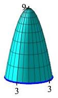
The graphic shows a circular paraboloid opening downward with z
between 0 and 9.

Clearly the curl of \(\vec{F}\) is ugly, but the boundary curve, which is the circle \(x^2+y^2=9\) for \(z=0\), is simple. Further, on the circle the vector field reduces to \[ \vec{F}=\langle-y,x,x^2+y^2\rangle \] which is also simple. So we want to use Stokes' Theorem and compute the line integral \(\displaystyle \oint_{\partial S} \vec{F}\cdot d\vec{s}\).
We first parametrize the circle as: \[ \vec{r}(\theta)=\vec R(3,\theta) =(3\cos\theta,3\sin\theta,0) \quad \text{for} \quad 0 \le \theta \le 2\pi \] We compute the tangent vector: \[ \vec{v}=\langle-3\sin\theta,3\cos\theta,0\rangle \] Since the surface is oriented out and up, the curve must be oriented counterclockwise which it is. On the circle the vector field is \[ \vec{F}=\langle-y,x,x^2+y^2\rangle =\langle-3\sin\theta,3\cos\theta,9\rangle \] So the integral is \[ \iint_S \vec{\nabla}\times\vec{F}\cdot d\vec{S} =\oint_{\partial S} \vec{F}\cdot d\vec{s} =\int_0^{2\pi} \vec{F}\cdot\vec{v}\,d\theta =\int_0^{2\pi} 9\,d\theta=18\pi \]

Use Stokes' Theorem to compute \(\displaystyle \iint_S \vec{\nabla}\times\vec{F}\cdot d\vec{S}\) for \(\vec{F}=\langle-y,x,x^2+y^2\rangle\) over the oscillating surface \(S\) shown at the right oriented upward, which may be parametrized by \(\vec{R}(r,\theta) =\langle r\cos\theta,r\sin\theta,r\sin(5\theta)\rangle\) for \(r\le2\).

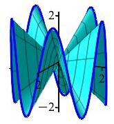
The graphic shows a saddle surface with 5 up and down oscillations
with the saddle point at the origin.

The boundary curve may be obtained by setting \(r=2\) in the surface \(\vec{R}(r,\theta)\). So: \[ \vec r(\theta)=\vec{R}(2,\theta) =\langle 2\cos\theta,2\sin\theta,2\sin(5\theta)\rangle \] Notice how \(x\) and \(y\) go around a circle while \(z\) oscillates up and down \(5\) times.

\(\displaystyle \oint_{\partial S} \vec{F}\cdot d\vec{s}=8\pi\)

Since we are told to use Stokes' Theorem, we convert the integral into the line integral \(\displaystyle \oint_{\partial S} \vec{F}\cdot d\vec{s}\) around the boundary. The boundary curve may be obtained by setting \(r=2\) in the surface \(\vec{R}(r,\theta)\). So: \[ \vec r(\theta)=\vec{R}(2,\theta) =\langle 2\cos\theta,2\sin\theta,2\sin(5\theta)\rangle \] The velocity is: \[ \vec v=\langle -2\sin\theta,2\cos\theta,10\cos(5\theta)\rangle \] Since the surface is oriented upward, the boundary must be traversed counterclockwise, which is the direction \(\vec v\) points. On the curve, the vector field becomes: \[ \vec{F}=\langle-y,x,x^2+y^2\rangle =\langle-2\sin\theta,2\cos\theta,4\rangle \] So their dot product is: \[ \vec{F}\cdot\vec v =4\sin^2\theta+4\cos^2\theta+40\cos(5\theta) =4+40\cos(5\theta) \] So the line integral is: \[ \oint_{\partial S} \vec{F}\cdot d\vec{s} =\int_0^{2\pi} [4+40\cos(5\theta)]\,d\theta =\left[\rule{0pt}{10pt}4\theta+8\sin(5\theta)\right]_0^{2\pi} =8\pi \]

Notice that by doing the line integral instead of the surface integral, we did not need to compute the curl of \(\vec F\), nor the normal vector to the surface, nor do a double integral instead of a single integral.

26. Stokes' Theorem

d. Applications

2. Converting Surface Integrals to Line Integrals

Heading