21. Multiple Integrals in Curvilinear Coordinates
a. Integrating in Polar Coordinates
3. Integral over a Non-Rectangular Polar Region
On the previous page, we learned how to integrate over a polar rectangle. Polar coordinates can also be used to compute integrals over some regions which are not polar rectangles, namely those of Type \(r\) or Type \(\theta\).
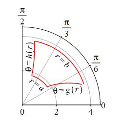
A region is of Type \(r\) if it consists of all points satisfying \(a \le r \le b\) and \(g(r) \le \theta \le h(r)\). A Type \(r\) integral is an integral over a region of Type \(r\).
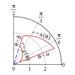
A region is of Type \(\theta\) if it consists of all points satisfying \(\alpha \le \theta \le \beta\) and \(g(\theta) \le r \le h(\theta)\). A Type \(\theta\) integral is an integral over a region of Type \(\theta\).xx
Samples of these regions are shown below:
We most often work with regions of type \(\theta\) because the boundaries \(r=g(\theta)\) and \(r=h(\theta)\) are standard polar curves. In Calculus 2, you may have learned that the area of a region of Type \(\theta\) is \(\displaystyle \dfrac{1}{2}\int_\alpha^\beta (h(\theta)^2-g(\theta)^2)\,d\theta\). If not, we will derive it on the next page from the 2D formula.
To compute double integrals over these types of regions we use the following theorems which say that the double integrals can be written as iterated integrals, with the area differential \[ dA=r\,dr\,d\theta \]
Memorize this!
If \(R\) is a Type \(r\) region with \(a \le r \le b\) and
\(g(r) \le \theta \le h(r)\), then
\[
\iint\limits_R f(r,\theta)\,dA
=\int_a^b\int_{g(r)}^{h(r)} f(r,\theta)\,r\,d\theta\,dr
\]
This is just the iterated integral computed by holding \(r\) fixed
while doing the \(\theta\) integral and then integrating the resulting
function over \(r\).
(Optional)
If \(R\) is a Type \(\theta\) region with \(\alpha \le \theta \le \beta\) and
\(g(\theta) \le r \le h(\theta)\), then
\[
\iint\limits_R f(r,\theta)\,dA
=\int_\alpha^\beta\int_{g(\theta)}^{h(\theta)} f(r,\theta)\,r\,dr\,d\theta
\]
This is just the iterated integral computed by holding \(\theta\) fixed
while doing the \(r\) integral and then integrating the resulting
function over \(\theta\).
(Optional)
Notice that, in both cases, the inner integral has limits that depend on the variable of the outer integral, but not vice versa. So you cannot, in general, reverse the order of integration. However, it is frequently useful to convert from rectangular coordinates to polar coordinates as done on another page.
In solving problems, it is usually sufficient to plot the base.
In practice, most polar integrals are for Type \(\theta\) regions. So we start with them:
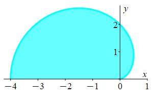
Find the volume under the surface \(z=y\) above the region in the \(xy\)-plane inside the cardioid \(r=2-2\cos\theta\) with \(y \ge 0\).
The plot shows the base of the solid.
This is a Type \(\theta\) region since \(0 \le \theta \le \pi\) and
\(0 \le r \le 2-2\cos\theta\). (Look at a radial line and see where it
crosses the curve.) In the integral for the volume, we express \(x\),
\(y\) and \(dA\) in polar coordinates:
\[\begin{aligned}
x=r\cos\theta &\qquad y=r\sin\theta \\
\text{and} \qquad &dA=r\,dr\,d\theta
\end{aligned}\]
So the volume is: \[\begin{aligned} V&=\iint\limits_R y\,dA =\int_0^\pi\int_0^{2-2\cos\theta} (r\sin\theta)\,r\,dr\,d\theta \\ &=\int_0^\pi\sin\theta \left[\dfrac{r^3}{3}\right]_{r=0}^{2-2\cos\theta}\,d\theta =\dfrac{1}{3}\int_0^\pi (2-2\cos\theta)^3\sin\theta\,d\theta \end{aligned}\] To do the integral, we make the substitution \(u=2-2\cos\theta\). Then \(du=2\sin\theta\,d\theta\) and \(\dfrac{1}{2}du=\sin\theta\,d\theta\). So: \[ V=\dfrac{1}{6}\int_0^4 u^3\,du =\dfrac{1}{6}\left[\dfrac{u^4}{4}\right]_0^4 =\dfrac{1}{6}4^3 =\dfrac{32}{3} \]
Find the area inside the spiral \(r=\theta\) for \(0\le\theta\le\pi\).
Recall: The area of a region is given by \(\displaystyle A=\iint1\,dA\).
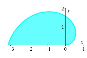
The Type \(\theta\) region is \(0\le r\le \theta\) for \(0\le\theta\le\pi\).
\(A=\dfrac{\pi^3}{6}\)
This is a Type \(\theta\) region. So the area is: \[\begin{aligned} A&=\iint1\,dA=\int_0^\pi\int_0^\theta 1\,r\,dr\,d\theta \\ &=\int_0^\pi\left[\dfrac{r^2}{2}\right]_0^\theta\,d\theta =\int_0^\pi\dfrac{\theta^2}{2}\,d\theta \\ &=\left[\dfrac{\theta^3}{6}\right]_0^\pi =\dfrac{\pi^3}{6} \end{aligned}\]
Type \(r\) integrals are uncommon, but here are some:
Find the area of the region bounded by the curves \(\theta=r\) and \(\theta=\dfrac{1}{2}(\pi-r)\) .
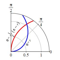
We cannot do this integral as a Type \(\theta\) integral because the \(\theta\) limits are not constant. So we do it as a Type \(r\) integral because the \(\theta\) bounds are already given as functions of \(r\). To find the bounds for \(r\), we first note that both curves pass through the origin. For the first curve the origin is \((r,\theta)=(0,0)\), but for the second curve, the origin is \((r,\theta)=\left(0,\dfrac{\pi}{2}\right)\). To find the other intersection point, we set the curves equal: \[ \dfrac{1}{2}\pi-\,\dfrac{1}{2}r=r \quad \Rightarrow \quad \dfrac{\pi}{2}=\dfrac{3}{2}r \quad \Rightarrow \quad r=\dfrac{\pi}{3} \] Thus, the \(r\)-bounds are: \(0 \le r \le \dfrac{\pi}{3}\). The graph confirms that the point of intersection is just past \(r=1\). Travelling counterclockwise (lower values to higher values) in the graph, the \(\theta\)-bounds are \(r \le \theta \le \dfrac{1}{2}(\pi-r)\). So the area is: \[\begin{aligned} \text{Area} &=\iint\limits_R 1\,dA =\int_0^{\pi/3}\int_r^{(\pi-r)/2} r\,d\theta\,dr \\ &=\int_0^{\pi/3} \left(\dfrac{\pi-r}{2}-r\right)r\,dr =\int_0^{\pi/3} \left(\dfrac{\pi}{2}r-\,\dfrac{3}{2}r^2\right)\,dr \\ &=\left[\dfrac{\pi r^2}{4}-\,\dfrac{r^3}{2}\right]_0^{\pi/3} =\dfrac{\pi}{4}\left(\dfrac{\pi}{3}\right)^2 -\,\dfrac{1}{2}\left(\dfrac{\pi}{3}\right)^3 \\ &=\pi^3\left(\dfrac{1}{36}-\,\dfrac{1}{54}\right) =\dfrac{1}{108}\pi^3 \end{aligned}\]
Find the mass of the region between the spiral \(\theta=r\) and the
curve \(\theta=r^2\) if the mass density is
\(\delta=r\theta\).
Recall: The mass of a region is given by
\(\displaystyle M=\iint\delta\,dA\) where \(\delta\) is the mass density
in the region.
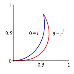
For \(0 \le r \le 1\), which is smaller: \(r\) or \(r^2\)?
\(\displaystyle M=\dfrac{1}{35} \)
This is an \(r\) integral because the bounds are given with \(\theta\) as functions of \(r\). We find the \(r\) bounds by equating the \(\theta\) bounds: \[ r=r^2 \quad \text{at} \quad r=0,1 \] Now, for \(0 \le r \le 1\), \(r^2\) is smaller than \(r\). So \(r^2\) is the lower bound. Therefore, the mass is: \[\begin{aligned} M&=\iint\delta\,dA =\int_0^1\int_{r^2}^r r\theta\,r\,d\theta\,dr \\ &=\int_0^1\left[\dfrac{\theta^2}{2}\right]_{r^2}^r r^2\,dr =\int_0^1\left(\dfrac{r^2}{2}-\dfrac{r^4}{2}\right)r^2\,dr \\ &=\left[\dfrac{r^5}{10}-\dfrac{r^7}{14}\right]_0^1 =\dfrac{1}{10}-\dfrac{1}{14}=\dfrac{1}{35} \end{aligned}\]
Try doing this integral as a \(\theta\) integral.
On the next page, we will use polar integrals in applications.
Heading
Placeholder text: Lorem ipsum Lorem ipsum Lorem ipsum Lorem ipsum Lorem ipsum Lorem ipsum Lorem ipsum Lorem ipsum Lorem ipsum Lorem ipsum Lorem ipsum Lorem ipsum Lorem ipsum Lorem ipsum Lorem ipsum Lorem ipsum Lorem ipsum Lorem ipsum Lorem ipsum Lorem ipsum Lorem ipsum Lorem ipsum Lorem ipsum Lorem ipsum Lorem ipsum