9. Line Integrals
g. Applications of Normal Line Integrals (Optional)
1. Expansion and Contraction
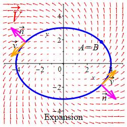
Let \(\vec V(x,y)\) be the velocity of a fluid at the point \((x,y)\) and let \(\vec r(t)\) be a closed curve.
Recall, the integral of the tangential component of \(\vec V\) \[ \oint_{\vec r} \vec V\cdot d\vec s =\oint_{\vec r} \vec V\cdot\hat v\,ds \] is the circulation of the fluid around the curve, as previously discussed.
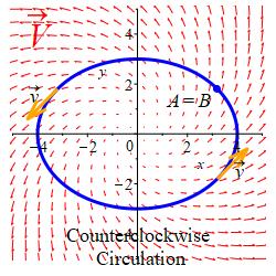
Also recall that if you look in the direction of \(\vec v\), then \(\vec n\) points along your right arm.
Consequently, if the curve is traversed counterclockwise, so that \(\hat n\) points outward, then the integral of the normal component of \(\vec V\) \[ \oint_{\vec r} \vec V\cdot d\vec n =\oint_{\vec r} \vec V\cdot\hat n\,ds \] is called the expansion of the fluid out of the curve \(\vec r(t)\).
On the other hand, if the curve is traversed clockwise, so that \(\hat n\) points inward, then the integral \(\displaystyle \oint_{\vec r} \vec V\cdot d\vec n\) is called the contraction of the fluid into the curve \(\vec r(t)\).
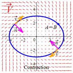
More generally, for any vector field \(\vec F\) the integral \(\displaystyle \oint_{\vec r} \vec F\cdot d\vec n\) is called the expansion (or contraction) of the vector field through the closed curve provided the curve is traversed counterclockwise (or clockwise, resp.).
If the expansion is positive or the contraction is negative, then the fluid is expanding. If the expansion is negative or the contraction is positive, then the fluid is contracting.
Find the expansion of the fluid velocity field \(\vec V=\langle 2x,3y\rangle\) through the circle \(x^2+y^2=16\).
We parametrize the circle by \(\vec r(\theta)=(4\cos\theta,4\sin\theta)\). Then the tangent vector is \(\vec v=\langle -4\sin\theta,4\cos\theta\rangle\) and the normal vector is \(\vec n=\langle 4\cos\theta,4\sin\theta\rangle\). This is outward since it is the same as the radius vector. The fluid velocity field along the curve is \[ \vec V=\langle 8\cos\theta,12\sin\theta\rangle \] Their dot product is \[\begin{aligned} \vec V\cdot\vec n &=32\cos^2\theta+48\sin^2\theta \\ &=16(1+\cos2\theta)+24(1-\cos2\theta) =40-8\cos2\theta \end{aligned}\] So the expansion is \[\begin{aligned} \text{Expansion}&=\int_0^{2\pi} \vec V\cdot\vec n\,d\theta =\int_0^{2\pi} (40-8\cos2\theta)\,d\theta \\ &=\left[40\theta-4\sin2\theta\rule{0pt}{10pt}\right]_0^{2\pi}=80\pi \end{aligned}\]
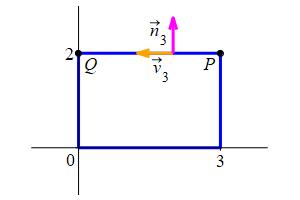
Find the expansion of the vector field \(\vec G=\langle2x+2y,3x-3y\rangle\) out of the rectangle \(0 \le x \le 3\) and \(0 \le y \le 2\). Integrate over the \(4\) edges and add them up.
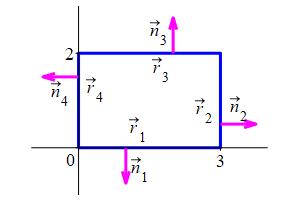
Traverse the rectangle counterclockwise. Parametrize each of the \(4\) edges using \(\vec r(t)=P+t\overrightarrow{PQ}\) where \(P\) and \(Q\) are the starting and finishing points of each edge. The plot shows \(P\) and \(Q\) for the edge \(\vec r_3\).
\(\text{Expansion}=-6\). Since the expansion is negative, the the vector field \(\vec G\) is contracting.
We parametrize each of the \(4\) edges, counterclockwise,
using \(\vec r(t)=P+t\overrightarrow{PQ}\) where \(P\) and \(Q\) are the
starting and finishing points of each edge. For each, the parameter range
is \(0 \le t \le 1\).
For each of the \(4\) edges, click the Plot button. Here are the endpoints,
parametrization, and tangent vector.
\(P=(0,0)\) \(Q=(3,0)\) \(\vec r_1=(3t,0)\)
\(\vec v_1=\langle 3,0\rangle\)
\(P=(3,0)\) \(Q=(3,2)\) \(\vec r_2=(3,2t)\)
\(\vec v_2=\langle 0,2\rangle\)
\(P=(3,2)\) \(Q=(0,2)\) \(\vec r_3=(3-3t,2)\)
\(\vec v_3=\langle -3,0\rangle\)
\(P=(0,2)\) \(Q=(0,0)\) \(\vec r_4=(0,2-2t)\)
\(\vec v_4=\langle 0,-2\rangle\)
For each of the \(4\) edges, here are the normal vector, the vector field \(\vec G=\langle2x+2y,3x-3y\rangle\) evaluated on the curve, and their dot product. \[\begin{aligned} \vec n_1&=\langle 0,-3\rangle &\vec G_1&=\vec G(3t,0)=\langle 6t,9t\rangle &\vec G_1\cdot\vec n_1&=-27t \\ \vec n_2&=\langle 2,0\rangle &\vec G_2&=\vec G(3,2t)=\langle 6+4t,9-6t\rangle &\vec G_2\cdot\vec n_2&=12+8t \\ \vec n_3&=\langle 0,3\rangle &\vec G_3&=\vec G(3-3t,2)=\langle 10-6t,3-9t)\rangle &\vec G_3\cdot\vec n_3&=9-27t \\ \vec n_4&=\langle -2,0\rangle &\vec G_4&=\vec G(0,2-2t)=\langle 4-4t,-6+6t\rangle &\vec G_4\cdot\vec n_4&=-8+8t \end{aligned}\] For each of the \(4\) edges, here is the normal line integral of \(\vec G\). \[\begin{aligned} \int_{\vec r_1} \vec G\cdot\,d\vec n &=\int_0^1 -27t\,dt=\left[\rule{0pt}{10pt}-\dfrac{27}{2}t^2\right]_0^1=-\dfrac{27}{2} \\ \int_{\vec r_2} \vec G\cdot\,d\vec n &=\int_0^1 12+8t\,dt=\left[\rule{0pt}{10pt}12t+4t^2\right]_0^1=16 \\ \int_{\vec r_3} \vec G\cdot\,d\vec n &=\int_0^1 9-27t\,dt=\left[\rule{0pt}{10pt}9t-\dfrac{27}{2}t^2\right]_0^1=-\,\dfrac{9}{2} \\ \int_{\vec r_4} \vec G\cdot\,d\vec n &=\int_0^1 -8+8t\,dt=\left[\rule{0pt}{10pt}-8t+4t^2\right]_0^1=-4 \end{aligned}\] Finally, we total the \(4\) integrals: \[ \text{Expansion} =\oint \vec G\cdot\,d\vec n =-\dfrac{27}{2}+16+-\,\dfrac{9}{2}-4=-6 \] The fact that the expansion is negative says that the vector field \(\vec G\) is contracting.
In the chapter on Green's Theorem we will learn a much easier way to compute the integrals in the last two problems.
Heading
Placeholder text: Lorem ipsum Lorem ipsum Lorem ipsum Lorem ipsum Lorem ipsum Lorem ipsum Lorem ipsum Lorem ipsum Lorem ipsum Lorem ipsum Lorem ipsum Lorem ipsum Lorem ipsum Lorem ipsum Lorem ipsum Lorem ipsum Lorem ipsum Lorem ipsum Lorem ipsum Lorem ipsum Lorem ipsum Lorem ipsum Lorem ipsum Lorem ipsum Lorem ipsum