1. Coordinate Systems

c. Polar Coordinates - 2D

4. 2D Polar Plots

Before you can graph polar curves, you need to understand the graphs of the basic trig functions and how to shift them. These are covered in the review chapter on Trigonometry.

You can also review graphs of the basic trig functions and how to shift them by using the following Maplets (requires Maple on the computer where this is executed):

Basic 6 Trigonometric FunctionsRate It

Shifting Trigonometric FunctionsRate It

Properties of Sine and Cosine CurvesRate It

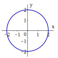
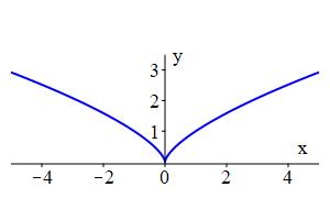
The rectangular graph of an equation is the set of all points whose rectangular coordinates \((x,y)\) satisfy the equation. For example, the graphs of the circle \(x^2+y^2=4\) and the cusp \(x^2=y^3\) are

Circle
The plot shows a circle with radius 2 centered at the origin.
Cusp
The plot shows a curve with a cusp at the origin that goes upwards to
    the left and right like the wings of a bird. They come to a sharp point
    at the origin.

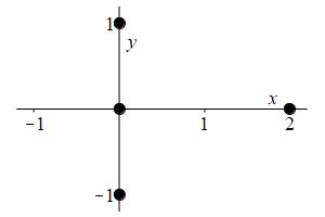
Similarly, the polar graph of a polar equation is the set of all points for which some pair of polar coordinates \((r,\theta)\) satisfy the equation. The simplest examples make one coordinate constant. For example, the graphs of the circle \(r=2\) and the ray (or line, if \(r\) can be negative) \(\theta=\dfrac{\pi}{6}\) are

Circle 
Ray 

In the graph of \(\theta=\dfrac{\pi}{6}\), if we require \(r \ge 0\), then the graph is only the blue ray. If we allow \(r \lt 0\), then the graph is the whole red and blue line.

We want to be able to graph more complicated polar equations. So let's do it by examples:

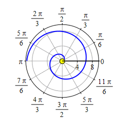
Plot the spiral \(r=\theta\).

We first graph the part of the curve with \(\theta \ge 0\). We start at \(r=\theta=0\) which is the origin. As \(r=\theta\) gets larger, we travel around counterclockwise and the radius also gets larger. So we trace out a spiral as shown in the first plot.

The video shows a blue counterclockwise spiral with a point starting
      at the origin and moving along the spiral.

As \(r=\theta\) gets negative, we travel around clockwise and since \(r\) is also negative, we measure \(|r|\) backwards, which traces out a spiral which is the mirror image through the \(y\)-axis of the first half as shown in the second plot.

The video shows the same blue counterclockwise spiral plus a red
      clockwise spiral which is a mirror image through the y axis of the
      blue spiral. A point starts at the far end of the red spiral, moves inward
      along that spiral and then outward along the blue spiral

If we restrict to the part of the curve, \(r=\theta\), with \(-\,\dfrac{3\pi}{2} \le \theta \le \dfrac{3\pi}{2}\), we get a heart shape.

Happy Valentine's Day!

The plot shows the piece of the 2 spirals in the previous plot
      between theta = minus 3 pi over 2 and plus 3 pi over 2. Together they
      form a heart shape for Valentines day.

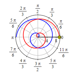
Plot the curve \(r=|\theta|\).

The plot shows two spirals going out from the origin which are mirror
    images through the x axis. There is also an animated point going outward
    from the origin along the first spiral and then inward along the second
    spiral back to the origin.

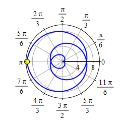
Start with the graph of \(r=\theta\) for \(\theta \ge 0\).

The video shows a point going out from the origin along a blue
      counterclockwise spiral.

Then take its mirror image through \(\theta=0\) which is the positive \(x\)-axis.

The plot shows the same spiral as in the first plot plus its miror
      image through the x axis. There is also an animated point going outward
      from the origin along the first spiral and then inward along the second
      spiral back to the origin.

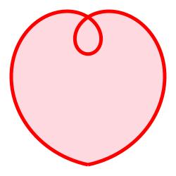
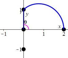
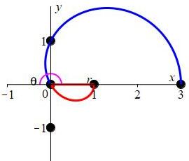
Plot the cardioid \(r=1+\cos{\theta}\).

First think of \(r\) and \(\theta\) as rectangular coordinates. The graph of \(r=\cos{\theta}\) is

The plot shows a cosine curve that starts at 1 for theta equals 0 
      then dips down to -1 at theta equals pi then goes back up to 1 at theta 
      equals 2 pi./>

We lift this up by \(1\) so that the graph of \(r=1+\cos\theta\) is

The plot shows the same cosine curve lifted up by one.
      It starts at 2 for theta equals 0 then dips down to 0 at theta equals pi
      and then goes back up to 2 at theta equals 2 pi.

We first plot the polar points for these interesting points:

\(\theta=\) \(0\) \(\dfrac{\pi}{2}\) \(\pi\) \(\dfrac{3\pi}{2}\) \(2\pi\)
\(r=\) \(2\) \(1\) \(0\) \(1\) \(2\)
The plot shows 4 dots, one at the origin, one at 0,1, one at dot at
      0,-1 and one at 2,0.

We now connect the dots in each quadrant. From the rectangular plot we see that as \(\theta\) increases from \(0\) to \(\dfrac{\pi}{2}\), the value of r decreases from \(2\) to \(1\). We add this to the plot:

The plot shows the dots from the previous plot as well as an arc
      in the first quadrant connecting from 2,0 to 0,1.

On the interval \(\dfrac{\pi}{2} \lt \theta \lt \pi\) we see that \(r\) decreases from \(1\) to \(0\). We add this section next:

The plot shows the dots and the curve from the previous plot as well
      as an arc from 0,1 to the origin.

Finally, we see that as \(\theta\) increases from \(\pi\) to \(\dfrac{3\pi}{2}\) to \(2\pi\), the value of \(r\) reverses and goes from \(0\) to \(1\) and finally back to \(2\). We conclude from this that the second half of the cardioid is a mirror image of the first. This finishes the plot:

The plot shows the dots and curves from the previous plot as well as 
      the mirror image of those curves through the x axis, forming a heart 
      shape with the cusp at the left.
Cardioid:   \(r=1+\cos\theta\)

Because it is shaped like a heart!

Watch the animation of the cardioid being drawn:

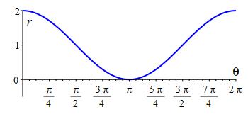
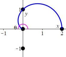
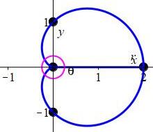
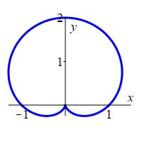
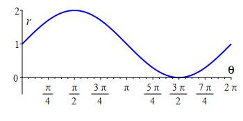
Plot the cardioid \(r=1+\sin{\theta}\).

Cardioid:   \(r=1+\sin\theta\)

The plot shows a cardioid with the cusp at the bottom.
The plot shows a sine curve lifted up by 1 that starts at 1 for
      theta equals 0 then goes up to 2 at theta equals pi over 2 then dips
      down to 0 at theta equals 3 pi over 2 then goes back up to 1 at theta
      equals 2 pi.
Cardioid:   \(r=1+\sin\theta\)

Frequently, when plotting polar functions we allow \(r\) to be negative by measuring backward. In particular, if the direction is \(\theta\), then

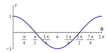
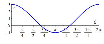
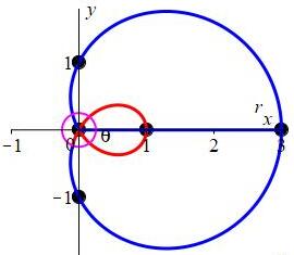
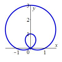
Plot the limaçon \(r=1+2\cos{\theta}\).

We follow the same procedure as last time by first graphing \(r\) as a function of \(\theta\) as rectangular coordinates:

The plot shows a sine curve stretched vertically by 2 and then
      lifted up by 1. It starts at 3 for theta equals 0 then dips down to -1
      at theta equals pi then goes back up to 3 at theta equals 2 pi.
      It crosses the x axis at 2 pi over 3 and at 4 pi over 3.

Notice that \(r=1+2\cos{\theta}=0\) when \(\cos{\theta}=-\,\dfrac{1}{2}\) or \(\theta=\dfrac{2\pi}{3}\) and \(\dfrac{4\pi}{3}\). We add these to our list of important points.

We plot the polar points at the important values of \(\theta\):

\(\theta=\) \(0\) \(\dfrac{\pi}{2}\) \(\dfrac{2\pi}{3}\) \(\pi\) \(\dfrac{4\pi}{3}\) \(\dfrac{3\pi}{2}\) \(2\pi\)
\(r=\) \(3\) \(1\) \(0\) \(-1\) \(0\) \(1\) \(3\)
The plot shows 5 dots. One at 3,0; one at 1,0; one at 0,0; one at 
      0,1; and one at 0,-1.

Notice that the origin occurs twice when \(\theta=\dfrac{2\pi}{3}\) and \(\dfrac{4\pi}{3}\). Also when \(\theta=\pi\), which is the negative \(x\)-axis, \(r=-1\) which we measure backwards along the positive \(x\)-axis. Be careful to check that you know how each of these points is plotted!

Next, we connect the dots by observing that \(r\) decreases from \(3\) to \(0\) on the interval \(0 \lt \theta \lt \dfrac{2\pi}{3}\). Also notice that \(r\) is negative on the interval \(\dfrac{2\pi}{3} \lt \theta \lt \dfrac{4\pi}{3}\), so we measure \(r\) opposite to the direction of \(\theta\) on this interval.

The result is plotted for \(0 \lt \theta \lt \pi\) with the curve in red when \(r\) is negative:

The plot shows the 5 dots from the previous plot as well as the
      part of the limacon for theta from 0 to pi which spirals from 3,0 to 0,1
      to 0,0 and finally to 1,0. The top half is blue to indicate the radius
      is measured positive from the origin. The bottom half is red to indicate
      the radius is measured negative (backwards) from the origin.

Finally, we note again that the second half is a mirror image of the first. Thus by symmetry our final plot is:

The plot shows the first half of the limacon from the previous plot 
      along with the second half which is its mirror image through the x axis.
      The outer loop is blue and the inner loop which is at the left is red.
Limaçon: \(r=1+2\cos\theta\)

Watch the animation of the limaçon being drawn.

The word limaçon is French for snail, but you can also remember that it looks like a lima bean.

Notice the curve and the radial line are blue when the radius is positive and red when the radius is negative.

Plot the limaçon \(r=1+2\sin\theta\)

Limaçon   \(r=1+2\sin\theta\)

The plot shows a limacon with the inner loop at the bottom.
      The outer loop passes through 0,3. The inner loop passes through 0,1.
The plot shows a sine curve stretched vertically by 2 and then
      lifted up by 1. It starts at 1 for theta equals 0,  goes up to 2 at
      theta equals pi over 2 then dips down to -1 at theta equals three pi
      over 2 then goes back up to 1 at theta equals 2 pi.
Limaçon   \(r=1+2\sin\theta\)

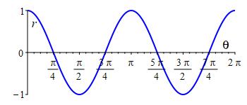
When there is a multiple of \(\theta\) inside the sine or cosine, the horizontal scale of the rectangular plot stretches or shrinks, changing the period.

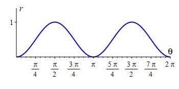
Plot the infinity curve \(r=\cos^2\theta=\dfrac{1+\cos2\theta}{2}\).

From the equation \(r=\cos^2\theta\), we find \(r=0\) when \(\theta=\dfrac{\pi}{2}\) or \(\dfrac{3\pi}{2}\) and \(r=1\) when \(\theta=0\) or \(\pi\). Also notice there are no negative values of \(r\). The equation \(r=\dfrac{1+\cos 2\theta}{2}\) makes it easier to plot. Here is a table of important values and a rectangular plot:

\(\theta=\) \(0\) \(\dfrac{\pi}{4}\) \(\dfrac{\pi}{2}\) \(\dfrac{3\pi}{4}\) \(\pi\) \(\dfrac{5\pi}{4}\) \(\dfrac{3\pi}{2}\) \(\dfrac{7\pi}{4}\) \(2 \pi\)
\(r=\) \(1\) \(0.5\) \(0\) \(0.5\) \(1\) \(0.5\) \(0\) \(0.5\) \(1\)
The plot shows a cosine curve shrunk horizontally and vertically by
      2 and raised by 1/2. It looks like a cosine curve that oscillates between
      1 and 0 with a period of pi, starting and ending at 1.

Notice the plot repeats with a period of \(\pi\). Here is the polar plot:

The plot shows an infinity curve, with the two loops on the left
      and right of the origin and going out to x equal 1 and -1.
Infinity:   \(r=\cos^2\theta\)

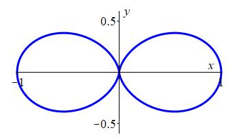
Plot the figure eight curve \(r=\sin^2\theta\).

Figure Eight:   \(r=\sin^2\theta\)

The video shows a figure eight curve being traced 
      out counterclockwise starting at 0,0 and tracing the top half and
      then the bottom half. There is also a number line with a
      point moving from 0 to 2 pi.

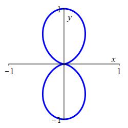
Here is a rectanguar plot, followed by the animated polar plot.

The plot shows a a curve that looks like a sine wave shifted up by 
      1 and shrunk by a horizontally and vertically by a factor of 2,
      oscillating between 0 and 1 with a period of pi, starting and ending at 0.
Figure Eight:   \(r=\sin^2\theta\)

Now let's combine a change of period with negative values of \(r\).

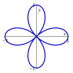
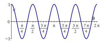
Plot the \(4\)-leaf rose \(r=\cos{2 \theta}\).

Notice that \(r=0\) when \(\theta=\dfrac{\pi}{4}, \dfrac{3\pi}{4}, \dfrac{5\pi}{4}\) or \(\dfrac{7\pi}{4}\). Also \(r=1\) when \(\theta=0\) or \(\pi\) and \(r=-1\) when \(\theta=\dfrac{\pi}{2}\) or \(\dfrac{3\pi}{2}\). Also note that the plot repeats with a period of \(\pi\). Here is a table of important values and a rectangular plot:

\(\theta=\) \(0\) \(\dfrac{\pi}{4}\) \(\dfrac{\pi}{2}\) \(\dfrac{3 \pi}{4}\) \(\pi\) \(\dfrac{5 \pi}{4}\) \(\dfrac{3\pi}{2}\) \(\dfrac{7 \pi}{4}\) \(2 \pi\)
\(r=\) \(1\) \(0\) \(-1\) \(0\) \(1\) \(0\) \(-1\) \(0\) \(1\)
The plot shows a cosine curve shrunk horizontally by a factor of 2.

Also notice that the plot has \(2\) positive bumps and \(2\) negative bumps in the interval \([0,2\pi]\). Here is the polar plot:

aria-label="The video shows a 4 leaf rose curve being traced out counterclockwise starting at 1,0 and tracing the top half of the right loop then the bottom loop then the left loop then the top loop and finally the bottom half of the right loop. On the right and left loops, the vector and curve are blue to indicate a positive radius. On the right and left loops, the vector and curve are red to indicate a negative radius. There is also a number line with a point moving from 0 to 2 pi.">
The plot shows the 4 leaf rose, with loops to the top, bottom, left and 
      right of the origin, going out to plus and minus 1 in the x and y 
      directions.
\(4\)-Leaf Rose:   \(r=\cos(2\theta)\)

In the animation, the radial line is blue when \(r\) is positive and red when \(r\) is negative. They trace out different leaves.

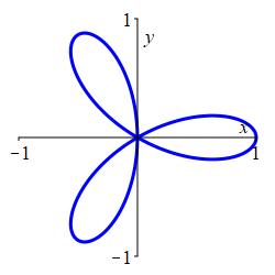
Plot the 3-leaf rose \(r=\cos{3 \theta}\)

3-Leaf Rose:   \(r=\cos(3\theta)\)

The plot shows a 3 leaf rose, with loops to the right and both up and 
      down to the left, going out 1 from the origin.

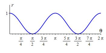
Here is a table of values and the rectangular plot:

\(\theta =\) \(0\) \(\dfrac{\pi }{6}\) \(\dfrac{\pi }{3}\) \(\dfrac{\pi }{2}\) \(\dfrac{2\pi }{3}\) \(\dfrac{5\pi }{6}\) \(\pi \)
\(r=\) \(1\) \(0\) \(-1\) \(0\) \(1\) \(0\) \(-1\)
The plot shows a cosine wave shrunk horizontally by a factor of 3.
3-Leaf Rose:   \(r=\cos(3\theta)\)

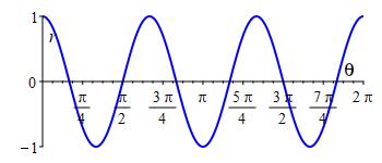
There are \(3\) positive bumps and \(3\) negative bumps in the interval \([0,2\pi]\). Here is the polar plot:

In the animation, the radial line is blue when \(r\) is positive and red when \(r\) is negative. Notice that each leaf of the rose is traced out twice, once when \(r\) is positive and once when \(r\) is negative.

How many leaves are there on the rose \(r=\cos(n \theta)\) if \(n\) is even? Why?

The rose \(r=\cos(n\theta)\) with even \(n\) has \(2n\) leaves, \(n\) with a positive radius and \(n\) with a negative radius.

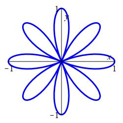
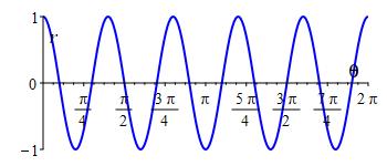
For example, the rose \(r=\cos(4\theta)\) has \(8\) leaves:

The plot shows a 8 leaf rose, with loops along the positive and
      negative x and y axes and along the positive and negative 45 degree lines,
      all with radius 1.
8-Leaf Rose:   \(r=\cos(4\theta)\)

The function \(\cos(n \theta)\) is \(1\) when the argument is a multiple of \(2\pi\), i.e. \(n \theta=2k\pi\). On the interval \(0 \le \theta \le 2\pi\), this is at \(\theta=\dfrac{2k\pi}{n}\) for \(k=1,2,\cdots,n\). These are the angles at the tip of each "positive" leaf. Notice that these are the even multiples of \(\dfrac{\pi}{n}\).

Similarly, on the interval \(0 \le \theta \le 2\pi\), we have \(\cos(n \theta)=-1\) when \(\theta=\dfrac{(2k+1)\pi}{n}\) for \(k=1,2,\cdots,n\). These are the angles at the tip of each "negative" leaf. However, since the radius is negative, the leaf actually occurs at: \[ \theta=\dfrac{(2k+1)\pi}{n}+\pi =\dfrac{(2k+1+n)\pi}{n} \] Since \(n\) is even, these are the odd multiples of \(\dfrac{\pi}{n}\).

All together, there are \(2n\) leaves \(n\) positive and \(n\) negative. For further evidence, the polar plot of \(r=\cos 4\theta \) has \(8\) leaves:

The plot shows a cosine wave shrunk horizontally by a factor of 4.
8-Leaf Rose:   \(r=\cos(4\theta)\)

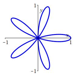
How many leaves are there on the rose \(r=\cos(n \theta)\) if \(n\) is odd? Why is this not the same answer as in the even case?

The rose \(r=\cos(n\theta)\) with odd \(n\) has \(n\) leaves. The \(n\) negative leaves coincide with the \(n\) positive leaves.

For example, the rose \(r=\cos(5\theta)\) has \(5\) leaves:

The plot shows a 5 leaf rose, with loops evenly spaced starting
      from the positive x axis attached together radially at the origin,
      all with radius 1.
5-Leaf Rose:   \(r=\cos(5\theta)\)

On the interval \(0 \le \theta \le 2\pi\), the function \(\cos(n \theta)\) is \(1\) when \(\theta=\dfrac{2k\pi}{n}\) for \(k=1,2,\cdots,n\). These are the angles at the tip of each "positive" leaf. Notice that these are the even multiples of \(\dfrac{\pi}{n}\).

Similarly, on the interval \(0 \le \theta \le 2\pi\), we have \(\cos(n \theta)=-1\) when \(\theta=\dfrac{(2k+1)\pi}{n}\) for \(k=1,2,\cdots,n\). These are the angles at the tip of each "negative" leaf. However, since the radius is negative, the leaf actually occurs at: \[ \theta=\dfrac{(2k+1)\pi}{n}+\pi =\dfrac{(2k+1+n)\pi}{n} \] Since \(n\) is odd, these are the even multiples of \(\dfrac{\pi}{n}\) which are at the same angles as the positive leaves.

All together, there are only \(n\) leaves. The \(n\) negative leaves coincide with the \(n\) positive leaves. For further evidence,the polar plot of \(r=\cos 5\theta \) has \(5\) leaves. The \(5\) negative leaves overwrite the \(5\) positive leaves.

The plot shows a cosine wave shrunk horizontally by a factor of 5.
5-Leaf Rose:   \(r=\cos(5\theta)\)

You can review the graphs and equations of polar curves and practice identifying polar curves from their graphs by using the following Maplets (requires Maple on the computer where this is executed):

Basic 14 Polar CurvesRate It

Identify a Polar Curve from its GraphRate It

© MY Math Apps

Supported in part by NSF Grant #1123255

NSF logo