10. Area and Average Value

d. Average Value and Mean Value Theorem

1. Average Value of a Function

Recall that to find the average of \(n\) numbers, \(f_1,f_2,\ldots,f_n\) we add the numbers and divide by \(n\): \[ f_\text{ave}=\dfrac{f_1+f_2+\cdots+f_n}{n} \]

Find the average value of a function \(f(x)\) on an interval \([a,b]\).

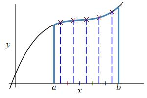
We first divide the interval into \(n\) subintervals each of width \(\Delta x=\dfrac{b-a}{n}\) and sample the function at a point \(x_i^*\) in the \(i^\text{th}\) interval giving the \(n\) numbers \(f(x_1^*),f(x_2^*),\ldots,f(x_n^*)\). The average of the function \(f(x)\) can be approximated by the average of these numbers: \[\begin{aligned} f_\text{ave} &\approx\dfrac{f(x_1^*)+f(x_2^*)+\cdots+f(x_n^*)}{n} \\ &\quad=\dfrac{1}{n}\sum_{i=1}^n\,f(x_i^*) \end{aligned}\]

This plot shows the graph of an increasing function in the first
quadrant with two vertial lines at x equals a and b which go from the x
axis up to the function. There are 4 short dashes on the x axis which
divide the interval from a to b into 5 equal pieces. Starting at the middle
of each piece, there is a vertical dashed line going up to the function.

We can approximate the average of the function \(f(x)=x^2\) on \([1,4]\) by dividing the interval into \(3\) subintervals and evaluating \(f(x)\) at the \(3\) midpoints: \[\begin{aligned} f(1.5)&=1.5^2=2.25 \\ f(2.5)&=2.5^2=6.25 \\ f(3.5)&=3.5^2=12.25 \end{aligned}\] and averaging to get \[ f_\text{ave}\approx\dfrac{2.25+6.25+12.25}{3}=6.917 \]

This plot shows the graph of an increasing function in the first
quadrant with two vertial lines at x equals 1 and 4 which go from the x
axis up to the function. There are 2 short dashes on the x axis at
x equals 2 and 3 which divide the interval into 3 equal pieces.
Starting at the middle of each piece, at x equals 1.5, 2.5 and 3.5,
there is a vertical dashed line going up to the function.

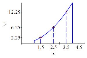
You will see in the next example that the correct average is \(f_\text{ave}=7\).

To get the exact average, we take the limit as \(n\rightarrow\infty\): \[ f_\text{ave} =\lim_{n\rightarrow\infty}\dfrac{1}{n} \sum_{i=1}^n f(x_i^*) \] This looks almost like the definition of an integral, except there is a \(\dfrac{1}{n}\) instead of a \(\Delta x\). To fix that, we multiply and divide by \(b-a\) and recall that \(\dfrac{b-a}{n}=\Delta x\): \[\begin{aligned} f_\text{ave} &=\dfrac{1}{b-a}\lim_{n\rightarrow\infty}\dfrac{b-a}{n} \sum_{i=1}^n f(x_i^*) \\ &=\dfrac{1}{b-a}\lim_{n\rightarrow\infty} \sum_{i=1}^n f(x_i^*)\Delta x \\ &=\dfrac{1}{b-a}\int_a^b f(x)\,dx \end{aligned}\]

Thus we conclude:

The average value of a function \(f(x)\) on an interval \([a,b]\) is: \[ f_\text{ave}=\dfrac{1}{b-a}\int_a^b f(x)\,dx \]

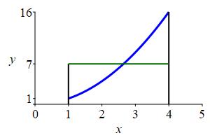
Find the average value of the function \(y=x^2\) on the interval \([1,4]\).

We have \(a=1\), \(b=4\) and \(b-a=3\). So \[\begin{aligned} f_\text{ave} &=\dfrac{1}{3}\int_1^4 x^2\,dx =\dfrac{1}{3}\left[\dfrac{x^3}{3}\right]_1^4 \\ &=\dfrac{1}{3}\left[\dfrac{64}{3}-\dfrac{1}{3}\right] =\dfrac{63}{9}=7 \end{aligned}\]

This plot shows an increasing function above the interval from 1 to 4.
There are two vertial lines at x equals 1 and 4, and a horizontal line
at y equals 7 which is the average value of this function.

Try it yourself:

Find the average value of the function \(y=(x-2)^2\) on the interval \([1,3]\).

The plot shows a parabola opening upward with vertex at x equals 2,
on the x axis. There are two vertial lines at x equals 1 and 3 specifing
the interval of this function.

\(\displaystyle f_\text{ave}=\dfrac{1}{2}\int_1^3 (x-2)^2\,dx=\dfrac{1}{3}\)

We have \(a=1\), \(b=3\) and \(b-a=2\). So \[\begin{aligned} f_\text{ave} &=\dfrac{1}{2}\int_1^3 (x-2)^2\,dx =\dfrac{1}{2}\left[\dfrac{(x-2)^3}{3}\right]_1^3 \\ &=\dfrac{1}{6}[1]-\dfrac{1}{6}[-1] =\dfrac{2}{6}=\dfrac{1}{3} \end{aligned}\]

This plot starts with the same plot as above and adds a horizontal line
at y equals one third above the x interval from 1 to 3 which
is the average value of this function.

On the next page, we will see a geometric interpretation of the average value in terms of area.

10. Area and Average Value

d. Average Value and Mean Value Theorem

1. Average Value of a Function

Heading