23. Riemann Sums, Integrals and the FTC

So far we have seen how to compute area using antiderivatives. However, mathematicians prefer to define area by filling the region with small pieces of area and adding them up.

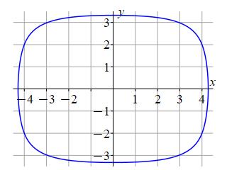
For example, consider the region at the right. In elementary school, you filled the region with squares.
The plot has \(44\) blue squares with area \(1\).
And possibly smaller pieces like triangles.
The plot has \(4\) yellow squares with area \(.5\).
Or even smaller pieces like little rectangles.
The plot has \(20\) red rectangles with area \(.25\).
And finally added them up: \[ \text{Area}\,\approx44\cdot1+4\cdot.5+20\cdot.25=51 \]

The graphic shows a rectangular
region with curved corners in the x y plane.

In this chapter, we will fill the region with vertical rectangles and add them up. These are called Riemann sums.

a1. Right Riemann Sums and Areas

To find the area, \(A(a,b)\), under the graph of \(y=f(x)\) above the \(x\)-axis between \(x=a\) and \(x=b\), follow these steps:

The graphic shows a
generic function defined in the first quadrant of the x y plane. The area
under the function and above the x axis between x = 2 and x = 14 is shaded. — In these plots, \(a=2\) and \(b=14\).

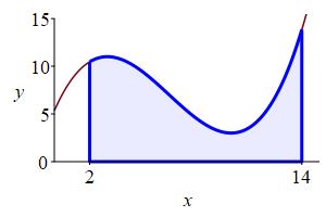
Divide the interval \([a,b]\) into \(n\) subintervals of equal width: \[ \Delta x=\dfrac{b-a}{n} \] Then the partition points are: \[ x_i=a+i\Delta x \qquad \text{for} \quad i=0,1,\cdots,n \] In particular: \[ x_0=a \qquad \text{and} \qquad x_n=b \] and for the \(i^\text{th}\) subinterval, the left endpoint is \(x_{i-1}\) and the right endpoint is \(x_i\).

The graphic is the same
as the previous graphic except the region under the function has now
been partitioned into six pieces of equal width. — Here, there are \(n=6\) partitions of width
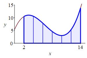
\(\Delta x=\dfrac{14-2}{6}=2\).
And the partition points are
\(2, 4, 6, 8, 10, 12, 14\).

Evaluate the function at the right endpoint of each subinterval and multiply by the width of the subinterval to get: \[ f(x_i)\Delta x \] This is the area of the \(i^\text{th}\) rectangle which is an approximation to the area under the curve above the \(i^\text{th}\) subinterval. Add these up for all the subintervals to get the Riemann sum: \[ \sum_{i=1}^n f(x_i)\Delta x \] which is an approximation to the area under the curve above \([a,b]\). The approximation gets better as \(n\) gets larger.

The graphic is the same
as the previous graphic except the six pieces have now been transformed
into six rectangles of equal width. The rectangles all begin on the x axis
and their heights are equal to the function value at their right
endpoints. — In this Riemann Sum, all \(6\) subintervals have
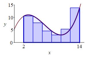
width \(\Delta x=2\) and the evaluation point
is the right endpoint of each interval.

Take the limit as the number of intervals, \(n\), goes to infinity. This is the definition of the area under the curve: \[ A(a,b) =\lim_{n\to\infty}\sum_{i=1}^n f(x_i)\Delta x \] The limit of a Riemann sum on the right is an example of an integral.

Here, the number of rectangles
starts at \(6\) and keeps doubling.

The (definite) integral of a function \(f(x)\) is the limit of the Riemann sums: \[ \int_a^b f(x)\,dx =\lim_{n\to\infty}\sum_{i=1}^n f(x_i)\Delta x \] Notation: The integral sign, \(\displaystyle \int\), (which is an elongated S for sum) replaces the limit of a sum. The differential, \(dx\), (previously discussed in the chapter on Differentials & Linear Approximation) replaces the change \(\Delta x\).

Thus the area under a curve is given by an integral:

If \(f(x)\) is positive, then the area under the graph of \(y=f(x)\) above the \(x\)-axis between \(x=a\) and \(x=b\) is: \[ A(a,b)=\int_a^b f(x)\,dx \]

The definitions of a Riemann sum and of an integral are actually more general and allow for functions, \(f(x)\), which are not necessarily positive, for partitions which are not necessarily evenly spaced and for evaluation points which are not necessarily the right endpoints. The full definition is given on the next page. However, for most purposes, the definitions on this page are totally sufficient.

Approximate the area below \(y=x^3\) above the \(x\)-axis between \(x=1\) and \(x=3\) using a Riemann sum with \(4\) equal width intervals and right endpoints.

The plot shows the graph of the
function y = x^3 in the first quadrant. The area under the function and
above the x-axis between x = 1 and x = 3 is shaded.

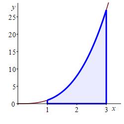
With \(n=4\) intervals, the width is: \[ \Delta x=\dfrac{3-1}{4}=0.5 \] The right endpoints are: \[ x_1=1.5 \quad x_2=2 \quad x_3=2.5 \quad x_4=3 \] and the function values are: \[\begin{aligned} f(1.5)&=3.375 & f(2)&=8 \\ f(2.5)&=15.625 & f(3)&=27 \end{aligned}\] So the Riemann sum is \[\begin{aligned} R_4&=3.375\cdot0.5+8\cdot0.5 \\ &\quad+15.625\cdot0.5+27\cdot0.5 \\ &=27.0 \end{aligned}\]

The graphic is the same as the
previous graphic except four rectangles of equal width have now been
overlayed over the area under the curve. The rectangles all begin on the
x axis and their heights are equal to the function value at their right
endpoints.

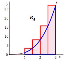
Here is an exercise on approximating an integral using right Riemann sums. An analogous exercise using Riemann sums with other evaluation points appears on the next page. The process of taking the limit is discussed on the page after next.

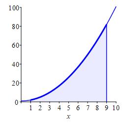
Approximate the integral \(\displaystyle \int_1^9(x^2+1)\,dx\) using:

The graphic shows the graph of the
function y = x^2 + 1 in the first quadrant. The area under the function and
above the x-axis between x = 1 and x = 9 is shaded.

\(4\) equal width subintervals and the right endpoints of each interval.

For equal width intervals \(\Delta x=\dfrac{b-a}{n}\). So: \(\displaystyle \int_a^bf(x)\,dx =\lim_{n\to\infty} \sum_{i=1}^n f(x_i)\Delta x\)

\(R_4=336\)

With \(n=4\) intervals, the width is \(\Delta x=\dfrac{9-1}{4}=2\). For right endpoints, the evaluation points are: \[ x_1=3 \quad x_2=5 \quad x_3=7 \quad x_4=9 \] and the function values are: \[\begin{aligned} f(3)=10 \qquad f(5)=26 \\ f(7)=50 \qquad f(9)=82 \end{aligned}\]

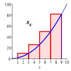
So the Riemann sum is \[ R_4=10\cdot2+26\cdot2+50\cdot2+82\cdot2=336 \]
\(8\) equal width subintervals and the right endpoints of each interval.

\(R_8=292\)

With \(n=8\) intervals, the width is \(\Delta x=\dfrac{9-1}{8}=1\). For right endpoints, the evaluation points are: \[\begin{aligned} x_1=2 \quad x_2=3 \quad x_3=4 \quad x_4=5 \\ x_5=6 \quad x_6=7 \quad x_7=8 \quad x_8=9 \end{aligned}\] and the function values are: \[\begin{aligned} f(2)=5\;\, \qquad f(3)=10 \\ f(4)=17 \qquad f(5)=26 \\ f(6)=37 \qquad f(7)=50 \\ f(8)=65 \qquad f(9)=82 \end{aligned}\]

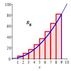
So the Riemann sum is \[ R_8=5+10+17+26+37+50+65+82=292 \]

In practice, one does not compute integrals using the Riemann sum formula. Rather, one uses this formula to derive the integral that needs to be computed in various applications (such as area, arc length and total mass). The integral is then computed using antiderivatives as prescribed by the Fundamental Theorem of Calculus: \[ \int_a^bf(x)\,dx=F(b)-F(a) \] as discussed later in this chapter.

23. Riemann Sums, Integrals and the FTC

a1. Right Riemann Sums and Areas

Heading