1. Coordinate Systems
c. Polar Coordinates - 2D
1. 2D Polar Coordinates
Rectangular coordinates \((x,y)\) are one way to specify a point, \(P\), in the plane, but they are not the only way. When we are studying circles, it is useful to use Polar Coordinates \((r,\theta)\) which identify the point, \(P\), using
- the radius \(r\) and
- the polar angle \(\theta\).
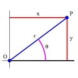
Like rectangular coordinates \(P=(x,y)\), the polar coordinates can be written as an ordered pair, \(P=(r,\theta)\). So you need to be careful to say whether this ordered pair is rectangular or polar.
Most often, the radius measures the (positive) distance from the origin, \(O\), to the point, \(P\), and the polar angle measures an angle (usually measured in radians and usually with \(0 \le \theta \lt 2\pi\)) counterclockwise from the positive \(x\)-axis to the ray \(\overrightarrow{OP}\).
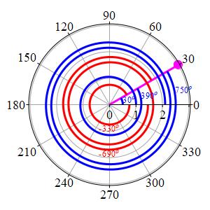
However, frequently the angle \(\theta\) is allowed to be bigger than \(2\pi\) or is allowed to be negative, in which case it is measured clockwise from the posiitve \(x\)-axis. Consequently, \(\theta\) is non-unique; we can always add or subtract an arbitrary multiple of \(2\pi\) or \(360^\circ\). Thus the point with polar coordinates \((3,{30^\circ})\) can also be written as \((3,{390^\circ})\), or \((3,{750^\circ})\), or \((3,{-330^\circ})\), or \((3,{-690^\circ})\) all of which are shown in the plot with blue angles positive and red angles negative.
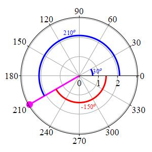
Further, once in a while, we allow \(r\) to be negative, for example in the context of solving equations or graphing. Then \(r\) is the negative of the distance from \(O\) to \(P\). When \(r\) is negative, the point \((r,\theta)\) is obtained by going a distance \(|r|\) along the ray at the angle \(\theta\pm\pi=\theta\pm180^\circ\). Think of this as going backwards along the ray at the angle \(\theta\). Thus the point with polar coordinates \((-3,{30^\circ})\) is actually the point \((3,{210^\circ})\) or \((3,-150^\circ)\).
Coordinate Curves
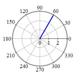
When you hold one of the coordinates fixed and let the other one vary, the point \(P=(r,\theta)\) traces out a coordinate curve. The curves are named by the coordinate which is changing.
When \(\theta\) is constant, you get a radial ray (assuming \(r \gt 0\)) called an \(r\)-curve, e.g. here is the \(r\)-curve with \(\theta=\dfrac{\pi}{3}\):
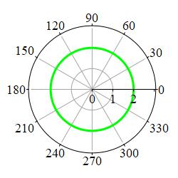
When \(r\) is constant, you get a circle called a \(\theta\)-curve, e.g. here is the \(\theta\)-curve with \(r=2\):
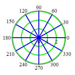
When you draw several coordinate curves of each type you get a coordinate grid. Here is a polar coordinate grid:
Heading
Placeholder text: Lorem ipsum Lorem ipsum Lorem ipsum Lorem ipsum Lorem ipsum Lorem ipsum Lorem ipsum Lorem ipsum Lorem ipsum Lorem ipsum Lorem ipsum Lorem ipsum Lorem ipsum Lorem ipsum Lorem ipsum Lorem ipsum Lorem ipsum Lorem ipsum Lorem ipsum Lorem ipsum Lorem ipsum Lorem ipsum Lorem ipsum Lorem ipsum Lorem ipsum