Search and Rank

This activity is based on the Google PageRank Algorithm developed by Larry Page.
An original version of this activity was developed for the TAMU SEE-Math Program in 2009 by David Kerr.

Repeatedly roll a die.
For the first roll, if it's 6 roll again. Otherwise, click on the photo of \[ 1 \to \,\text{Augustine} \quad 2 \to \,\text{Bernhard} \quad 3 \to \,\text{Carl} \quad 4 \to \,\text{David} \quad 5 \to \,\text{Emmy} \] For subsequent rolls, go to the page indicated on the previous page.
Keep track of the pages you visit by putting a tick mark on a piece of paper.
Can you predict the fraction of the time you will visit each page?

Here are some ways you can think about it:

Each student (or pair of students) in a class should visit 50-100 websites. The class should total the results from everyone in the class and divide by the total number of visits to all the websites. This will give the fraction of the visits that were made to each site. This is also called the probability of visiting each site.

Each student should divide their own number of visits to each site by the total number of their visits. Their fractions should be similar to those for the whole class.

These results are experimental. We would like to have a theoretical derivation.

The probabilities should be approximately: \[ P_A\approx 8.97\% \quad P_B\approx18.13\% \quad P_C\approx30.65\% \quad P_D\approx15.33\% \quad P_E\approx26.92\% \]

Here is a talley sheet where the individual students can talley their visits.

Here is an Excel spreadsheet where the class can total the results from the individual students.\(\rule[-5pt]{0pt}{10pt}\)
Enter the results from individual students in columns D, E, F, ... . The totals will appear in column B and the probabilities (as percents) will appear in column C.

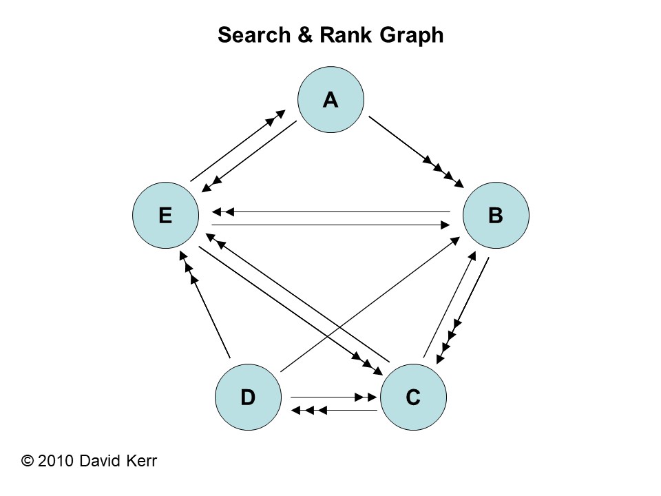
Draw a weighted directed graph with vertices and edges.
Which site to you think is visited the most, the least? Why?

The graph has one vertex (point) for each website people can visit.
The edges (lines) are the links people can follow between websites.
The graph is directed because each edge is marked by an arrow to show the direction it is followed.
The graph is weighted because each edge is marked by a number of arrows to say the probability that people will follow that edge.

SearchRankGraph

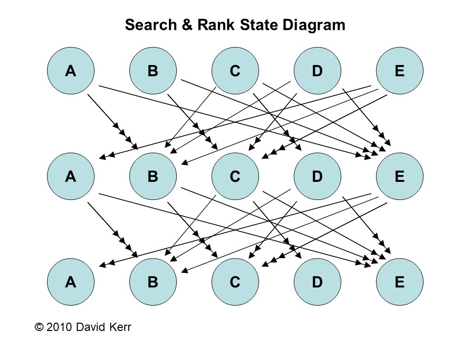
Draw a state diagram indicating how people move from one state to the next.

A state diagram consists of
1) two rows of vertices (points) with each row having one vertex for each website, and
2) arrows from the first row to the second row to indicate how people move from one website to the next.
The rows and arrows may be repeated to indicate how people move on subsequent steps.

SearchRankState

Construct a probability transition matrix which moves one state vector into the next.
What can you say about the sum of the numbers in each column? Why?

A state is the number or fraction of people visiting each website at one instance of time (a step). It is written as a column of numbers called the state vector.
A probability transition matrix is the matrix you multiply the state vector by to get the state at the next step.
Find the entries in the probability transition matrix.

\[ M=\begin{pmatrix} 0 &0 &0 &0 &\dfrac{1}{3} \\[8pt] \dfrac{2}{3} &0 &\dfrac{1}{6} &\dfrac{1}{6} &\dfrac{1}{6} \\[8pt] 0 &\dfrac{2}{3} &0 &\dfrac{1}{3} &\dfrac{1}{2} \\[8pt] 0 &0 &\dfrac{1}{2} &0 &0 \\[8pt] \dfrac{1}{3} &\dfrac{1}{3} &\dfrac{1}{3} &\dfrac{1}{2} &0 \end{pmatrix} \] The numbers in each column must add up to \(1\) because the people at each website must go somewhere.

Let \(a_0\), \(b_0\), \(c_0\), \(d_0\) and \(e_0\) be the number of people initially visiting website \(A\), \(B\), \(C\), \(D\) and \(E\), resp. Similarly, let \(a_1\), \(b_1\), \(c_1\), \(d_1\) and \(e_1\) be the number of people visiting website \(A\), \(B\), \(C\), \(D\) and \(E\), after \(1\) click. So the state vectors are: \[ \vec S_0= \begin{pmatrix} a_0 \\ b_0 \\ c_0 \\ d_0 \\ e_0 \end{pmatrix} \quad \text \quad \vec S_1= \begin{pmatrix} a_1 \\ b_1 \\ c_1 \\ d_1 \\ e_1 \end{pmatrix} \] Assuming the dice rolls are fair, then these are related by: \[ \vec S_1=M\vec S_0 \] where \(M\) is the propability transition matrix. Fill in the blanks below for the probability transition matrix. \[ \begin{pmatrix} a_1 \\ b_1 \\ c_1 \\ d_1 \\ e_1 \end{pmatrix} = \begin{pmatrix} \rule{.25in}{1pt} &\rule{.25in}{1pt} &\rule{.25in}{1pt} &\rule{.25in}{1pt} &\rule{.25in}{1pt} \\ \rule{.25in}{1pt} &\rule{.25in}{1pt} &\rule{.25in}{1pt} &\rule{.25in}{1pt} &\rule{.25in}{1pt} \\ \rule{.25in}{1pt} &\rule{.25in}{1pt} &\rule{.25in}{1pt} &\rule{.25in}{1pt} &\rule{.25in}{1pt} \\ \rule{.25in}{1pt} &\rule{.25in}{1pt} &\rule{.25in}{1pt} &\rule{.25in}{1pt} &\rule{.25in}{1pt} \\ \rule{.25in}{1pt} &\rule{.25in}{1pt} &\rule{.25in}{1pt} &\rule{.25in}{1pt} &\rule{.25in}{1pt} \\ \end{pmatrix} \begin{pmatrix} a_0 \\ b_0 \\ c_0 \\ d_0 \\ e_0 \end{pmatrix} \] As you fill in the blanks, think about the following situations. How do you produce these using a matrix multiplication?
1) Suppose there are initially \(6\) people visiting site \(B\). After they roll the die and click, how many people will then be at each site?
2) Suppose there are initially \(b_0\) people visiting site \(B\). After they roll the die and click, how many people will then be at each site?

Notice that the numbers in each column must add up to \(1\) because the people at each website at one step must go somewhere on the next step.

Simulate a series of steps by starting with the state vectors: \[ \vec S_0= \begin{pmatrix} 1 \\ 0 \\ 0 \\ 0 \\ 0 \end{pmatrix} \] and multiplying by the probability transition matrix some large number of times. Repeat this but start with state vectors with a \(1\) in a different positions.
Feel free to use a computer algebra system (such as Maple™) to do the matrix multiplications.
What do you notice about the final state vectors after 100 steps with different initial state vectors?
What do you notice about the final state vectors after 100 or 101 steps?

\[ \vec S_1=M\vec S_0 \qquad \vec S_2=M\vec S_1 \qquad \vec S_3=M\vec S_2 \qquad \cdots \qquad \vec S_n=M^n\vec S_0 \qquad \cdots \] You may understand what is going on better if you start with the state vector \[ \vec S_0= \begin{pmatrix} 36 \\ 0 \\ 0 \\ 0 \\ 0 \end{pmatrix} \] so that \(36\) people are moving around the websites.

Here is a Maple™ worksheet withn the correct probability transition matrix and the final state vector.

Here is a Maple™ worksheet that may help you do the computations. You can modify the probability transition matrix, the initial state vector and the number of steps.

Notice you get the same final state vector whether you do 100 or 101 steps and no matter which initial state vector you use.

You should have noticed that you get the same final state vector after a large number of steps no matter how many step you use and no matter which initial state vector you use (as long as the total probability in the initial state is \(1\)). Call this final state vector \[ \vec S_\infty= \begin{pmatrix} a \\ b \\ c \\ d \\ e \end{pmatrix} \] Since it does not change from step to step, it is called a steady state solution. It satisfies \[ \vec S_\infty=M\vec S_\infty \] Use these equations to solve for \(a\), \(b\), \(c\), \(d\) and \(e\).
This appears to be 5 equations for 5 unknowns. However, the sum of the 5 equations is the trivial statement \(a+b+c+d+e=a+b+c+d+e\). So it is really only 4 equations for 5 unknowns. We need a 5\(^\text{th}\) equation. It is that the total probability is \(1\), i.e. \(a+b+c+d+e=1\). (This is called the normalization condition.)

xxx

\[ a=.0897 \quad b=.1813 \quad c=.3065 \quad d=.1533 \quad e=.2692 \]

The matrix equation is: \[ \begin{pmatrix} a \\[12pt] b \\[12pt] c \\[12pt] d \\[12pt] e \\[2pt] \end{pmatrix} =\begin{pmatrix} 0 &0 &0 &0 &\dfrac{1}{3} \\[8pt] \dfrac{2}{3} &0 &\dfrac{1}{6} &\dfrac{1}{6} &\dfrac{1}{6} \\[8pt] 0 &\dfrac{2}{3} &0 &\dfrac{1}{3} &\dfrac{1}{2} \\[8pt] 0 &0 &\dfrac{1}{2} &0 &0 \\[8pt] \dfrac{1}{3} &\dfrac{1}{3} &\dfrac{1}{3} &\dfrac{1}{2} &0 \end{pmatrix} \begin{pmatrix} a \\[12pt] b \\[12pt] c \\[12pt] d \\[12pt] e \\[2pt] \end{pmatrix} \] The component equations are: \[\begin{aligned} a&=\dfrac{1}{3}e \\ b&=\dfrac{2}{3}a+\dfrac{1}{6}c+\dfrac{1}{6}d+\dfrac{1}{6}e \\ c&=\dfrac{2}{3}b+\dfrac{1}{3}d+\dfrac{1}{2}e \\ d&=\dfrac{1}{2}c \\ e&=\dfrac{1}{3}a+\dfrac{1}{3}b+\dfrac{1}{3}c+\dfrac{1}{2}d \end{aligned}\] The first and fourth equations say \[ a=\dfrac{1}{3}e \quad \text{and} \quad d=\dfrac{1}{2}c \] We use these to eliminate \(a\) and \(d\) from the other three equations: \[\begin{aligned} b&=\dfrac{2}{9}e+\dfrac{1}{6}c+\dfrac{1}{12}c+\dfrac{1}{6}e &&=\dfrac{1}{4}c+\dfrac{7}{18}e \\ c&=\dfrac{2}{3}b+\dfrac{1}{6}c+\dfrac{1}{2}e \\ e&=\dfrac{1}{9}e+\dfrac{1}{3}b+\dfrac{1}{3}c+\dfrac{1}{4}c &&=\dfrac{1}{9}e+\dfrac{1}{3}b+\dfrac{7}{12}c \end{aligned}\] The first equations says \[ b=\dfrac{1}{4}c+\dfrac{7}{18}e \] We use this to eliminate \(b\) from the remaining two equations: \[\begin{aligned} c&=\dfrac{2}{3}\left(\dfrac{1}{4}c+\dfrac{7}{18}e\right)+\dfrac{1}{6}c+\dfrac{1}{2}e &&=\dfrac{1}{3}c+\dfrac{41}{54}e \\ e&=\dfrac{1}{9}e+\dfrac{1}{3}\left(\dfrac{1}{4}c+\dfrac{7}{18}e\right)+\dfrac{7}{12}c &&=\dfrac{2}{3}c+\dfrac{13}{54}e \\ \end{aligned}\] We now subtract the left side from the right side of each equation: \[\begin{aligned} 0&=-\,\dfrac{2}{3}c+\dfrac{41}{54}e \\ 0&=\dfrac{2}{3}c-\dfrac{41}{54}e \\ \end{aligned}\] These two equations say the same thing. So we throw one away and solve for \(c\): \[ c=\dfrac{3}{2}\dfrac{41}{54}e=\dfrac{41}{36}e \] We are now ready to use the normalization condition. We first plug in \(a\), \(d\) and \(b\) and simplify. Then we plug in \(c\) and solve for \(e\). \[\begin{aligned} a+b+c+d+e&=1 \\ \dfrac{1}{3}e+\left(\dfrac{1}{4}c+\dfrac{7}{18}e\right)+c+\dfrac{1}{2}c+e&=1 \\ \dfrac{7}{4}c+\dfrac{31}{18}e&=1 \\ \dfrac{7}{4}\left(\dfrac{41}{36}e\right)+\dfrac{31}{18}e&=1 \\ \dfrac{535}{144}e&=1 \\ e&=\dfrac{144}{535} \\ \end{aligned}\] Finally we substitute back. Since the rational numbers have become too complicated, we switch to decimals. \[\begin{aligned} e&=\dfrac{144}{535}\approx.26916 \\ c&=\dfrac{41}{36}e\approx\dfrac{41}{36}.26916\approx.30654 \\ b&=\dfrac{1}{4}c+\dfrac{7}{18}e \approx\dfrac{1}{4}.30654+\dfrac{7}{18}.26916\approx.18131 \\ d&=\dfrac{1}{2}c\approx\dfrac{1}{2}.30654\approx.15327 \\ a&=\dfrac{1}{3}e\approx\dfrac{1}{3}.26916\approx.08972 \end{aligned}\] In summary: \[ a=.08972 \quad b=.18131 \quad c=.30654 \quad d=.15327 \quad e=.26916 \] These agree with the answers to exercises 1 and 5. Notice they add up to \(1\) as required.

This question shows that if you know the probability transition matrix, then you can find the steady state solution by solving a system of equations instead of doing \(100\) matrix multiplications.

Search and Rank

Search and Rank

Heading